Image Enhancement by Histogram Manipulation

     Image can be enhanced by manipulating its histogram values.  This is what our activity is about.  So, let us go through the steps.

     First thing to do is to pick an image.  Figure 1 shows the image I used for this activity. Then, get the histogram of the image. To do this, I converted the image into grayscale and used the tabul() function in Scilab and get the number of the pixels ranging from 0 to 1.  Figure 2 shows the normalized histogram of the image.  From this normalized histogram, the cumulative distribution function was obtained using the function cumsum(), as shown in Figure 3.

Figure 1. A roundabout with a fountain sits between old buildings in Manila

(image taken here.)

Figure 2.  Probability Distribution Function (PDF) of the grayscaled image in 

Figure 1.

Figure 3.  Cumulative Distribution Function (CDF) of the

histogram in Figure 2.

     Now, using the technique called backprojecting, we would modify the image.  Based on the pixel values of the image, which is ranging from 0 to 1, we would create our desired CDF.  We would try first a linear CDF, as shown in Figure 4. Then, we would find the corresponding pixel values of the image to the desired CDF.  Using the function interp1(), the pixel values of the image were interpolated to its CDF.  Then, its output is interpolated again to the desired CDF.  This then gives the modified image, as shown in Figure 5.  It can be seen that the image has a darker tone.

Figure 4. Desired CDF (linear).

Figure 5. Histogram equalized image (linear CDF).

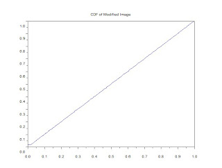
     To check if we have done the right thing, the CDF of the modified image should correspond to the desired CDF.  Figures 6 shows the CDF and the PDF of the modified image, respectively.

Figure 6 (a)

Figure 6 (b)

Figure 6. CDF (a) and PDF (b) of the modified image in Figure 5.

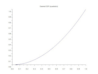
     Desired CDFs such as the quadratic and logarithmic functions were also tried.  Figure 7 shows the desired CDF for the two.

Figure 7 (a)

Figure 7 (b)

Figure 7.  Desired CDFs: quadratic (a), and logarithmic (b).

     Then, repeating the steps for backprojecting, the modified images were obtained, as shown in Figure 8.  It could be seen that the modified image from the quadratic CDF is lighter than the linear and logarithmic CDF.  The modified image from the logarithmic is the darkest of them all.

Figure 8 (a)

Figure 8 (b)

Figure 8.  Output images for quadratic CDF (a) and logarithmic CDF (b).

     To check, the CDF and PDF were again obtained for the modified images.

Figure 9 (a) CDF of the modified image (quadratic).

Figure 9 (b) PDF of the modified image (quadratic).

Figure 9 (c) CDF of the modified image (logarithmic).

Figure 9 (d) PDF of the modified image (logarithmic)

Figure 9.  The CDF and PDF of the modified images for the quadratic and logarithmic CDFs.

   Free software, such as GIMP, also allows you to modify the image by histogram manipulation.  To do this, open your image in GIMP then click IMAGE and choose the MODE as grayscale.  Then, go to COLORS and click CURVES.  Here, you can manipulate the histogram by dragging the line.  Figure 10 shows the manipulated histogram and the modified image using GIMP.

Figure 10 (a) Manipulated histogram.

Figure 10 (b) Modified image using GIMP's histogram manipulation.

Figure 10.  Manipulated histogram curve and the corresponding image output.

     I would like to thank Ma'am Jing and Joseph Raphael Bunao for clarifying important points to me.  I had trouble figuring out the correct algorithm for the backprojection of the image.

     I would give myself a score of 8/10.