Playing Notes by Image Processing

     The goal of this activity is to use image processing techniques to extract musical notes from a scanned music sheet and play it in Scilab. I used the music sheet for "Twinkle Twinkle Little Star" as shown in figure 1. 

     The problem to answer is how to detect the types of notes and the pitch level.

Now, let us go through the steps of the method used. :)

Figure 1.  Music sheet used in the activity.

A.  Detection of the types of notes.

     First, I cropped the image such that all the notes are in the same music lines.  Then, I reverted the color since functions in Scilab treat pixels with 0 value as background and 1 as foreground.  Figure 2 shows the  image.

Figure 2.  Music notes arranged along same lines.

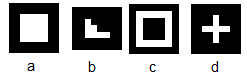
     Next, I made a template image for the quarter note, as shown in figure 3.  The correlation of the music notes with the quarter note will be taken.  This would give an image that will have high pixel values on points where there is high correlation.  The resulting image was then converted into a binary image, with a threshold value of 0.6.  This step hopes to filter out those with low correlation value. Figure 4 shows the correlation of the quarter note and its thresholded version.

Figure 3.  Template image used to detect quarter notes.

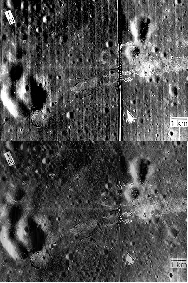
Figure 4a.  Correlation image of the quarter note to the rest of the notes in the music sheet.

Figure 4b.  Thresholded version of the correlation.

Figure 4.  Correlation of the quarter note to the rest of the notes

and its thresholded version.

     I noticed that at points where there is a quarter note, the blobs are bigger than at points where there are half notes.  Well, this is expected since the correlation is higher where there are quarter notes.  Instead of completely eliminating blobs for the half notes, I utilized the difference in sizes of the blobs for the quarter and half notes.  Using bwlabel(), I gained access to each blob and differentiated them based on their sizes.  But the problem with bwlabel() is that its tagging of the blobs is jungled up and not in order.  So to fix this, I obtained the x coordinate of each blob.  In matrix terms this would be the column where the blob lies.  I obtained the first column where the blob is, and using lex_sort() I arranged them in increasing order.  Now, I have obtained the note types in the music sheet. :)  I gave the half note a value of 0.5s and the quarter note is 0.75s.  Note that choosing the appropriate values for the time is very important.  Poor choice of time values will alter the melody and the resulting sound will be out of tune.

B.  Detection of the pitch level.

     The next task is to detect the pitch level.  Since the pitch is indicated by the vertical position of the notes on the music sheet, the y position of the blobs will be obtained.  In matrix terms, this would be the row on which the blob lies.  I obtained the largest value of the row for each blob as the indicator of the pitch.  Then, based on the image, I obtained their corresponding pitch.  The following shows the range of the row values for each pitch.

C = 40-43

D = 36-39

E = 33-35

F = 31-32

G = 25-28

A = less than 24

     From these values, I was able to differentiate the pitch of each notes.  I also applied the sorting technique used earlier to arrange the pitch correctly.  Now that I have the note types and the pitch levels, the next step is to make Scilab sing. :)

 C.  Making Scilab "sing"

     In Scilab, a sinusoid function was used to make sound.  The frequencies used were the corresponding frequencies of the pitch levels.  The function soundsec() was used to indicated how long the sound for that particular pitch would be.  And using sound(), the melody was played.  I used wavwrite() to save the sound file. :)

     To answer the question in the manual, set the frequency to zero when adding rests in the sound matrix.  Zero frequency means no vibration, therefore there would also be no sound.  

      This activity is the hardest for me.  I thought I'm not going to finish this.  But now that I did, it feels so great. hehe. :)

     I would like to thank Arvin Mabilangan for sharing his insights about this activity.  It really helped a lot.  I would give myself a score of 10/10 for successfully making Scilab sing with the correct notes and pitch. :)

 Click this link!!! Twinkle Twinkle Little Star

References:

[1] music sheet:

www.mamalisa.com/images/scores/twinkle_twinkle_little_star.jpg

[2] frequencies

http://www.seventhstring.com/resources/notefrequencies.html

[3] pitch levels

http://library.thinkquest.org/15413/theory/note-reading.htm

Color Image Processing

     Ever wondered what does the white balance setting in your camera means? Aside from using it to add special effects on the image, it is used to get the correct color of objects on the images that is on different light conditions.  In this activity, the different white balancing settings of a camera will be explored.  Then, images with wrong white balance settings will be corrected using two algorithms: the white patch and the gray world algorithm.

     Figure 1 shows images of colored paper clips with a white background taken under different lighting conditions.  The available white balance settings on the camera used are automatic, daylight, fluorescent, and tungsten.  These settings refer to the lighting conditions on which it must be used.  For the images taken inside a room with a fluorescent lighting, daylight and tungsten settings are not the appropriate settings (although it is not obvious for the daylight setting).  For images taken under natural light, the incorrect settings are fluorescent and tungsten.  For those taken directly under the sun, the incorrect settings are also fluorescent and tungsten.     Notice that the white background on the images with incorrect settings is not white at all.  For daylight, it is slightly yellow, for fluorescent and tungsten it is bluish. 

Figure 1a.  Image taken inside a room with a fluorescent lighting.

Figure 1b.  Image taken under natural lighting.

Figure 1c. Image taken under the morning sun (10:30am).

Figure 1.  A set of paper clips taken on different lighting conditions and white balance camera settings.

     To make the white background appear white for the wrongly white balanced images, white patch and gray world algorithm will be used. The white patch algorithm divides the RGB values of the image with the RGB values of the known white object.  This white balances the image.  For the gray world algorithm, the assumption is that the average color of the world is gray.  The balancing constants are the average of the RGB values of the image.  The RGB values are divided by these constants to white balance the image.  To prevent image saturation, the maximum pixel value were cut-off to 1.

Figure 2a.  Daylight white balance setting.

Figure 2b.  Tungsten white balance camera setting.

Figure 2.  Images taken inside a room with tungsten lighting.

 

Figure 3a.  Fluorescent white balance setting.

Figure 3b.  Tungsten white balance setting.

Figure 3.  Images taken outside a room with natural lighting.

Figure 4a.  Fluorescent white balance setting.

 Figure 4.  Images taken directly under the sun.

     The results show even white balancing for the white patch algorithm, while for the gray world algorithm there are apparent shades.  There are also some regions in the gray world white balanced images where the white background is still not white.  To compare the two algorithms further, objects with the same hue were imaged using a wrong white balance setting.  For this case, red hue was chosen and the image was taken under natural light and using tungsten as the white balance setting.

Figure 5.  Comparison of the white patch and gray world algorithm.

      It can be seen that the use of white patch algorithm showed better white balancing of the image compared to the gray world algorithm.  This result is also consistent with the results for different lighting conditions and camera white balancing settings.

     I would like to thank Dennis Ivan Diaz and Ma'am Jing for the helpful discussions.  I would give myself a grade of 9/10.  Although the required outputs are presented, the image quality was not that good because only a camera phone was used in this activity.

Color Image Segmentation

     Color image segmentation is very useful in separating parts of the images when the gray level values of the region of interest (ROI) is almost the same as the background.  Figure 1 shows an image of a red bell pepper that will be used in this activity.  The goal is to separate the red bell pepper from the background.  Can it be done using thresholding of the gray level values?  Let's see. :)

     The histogram of the gray level image was obtained, as shown in figure 3.  Since the bell pepper has darker tones than the rest of the image, its pixel values are expected to be near 0.  Based on the histogram values, the image was converted into a binary image with a threshold of 0.3.  Figure 4 shows the resulting image.  Though some parts of the bell pepper are apparent, it is not entirely separated from the background since some part of its leaves are also apparent.  Is there a better way????

     In fact, there is. :)

     Notice that the image has differing brightness of the same color.  For better representation of the color space, brightness is separated from the hue.  This can be done by normalizing the RGB values per pixel.  The normalized RGB values can be used to know the chromaticity of the ROI and consequently use it to discriminate the ROI from the background.

     In this activity, parametric and non-parametric probability distribution will be used as the criteria for segmenting the image.

Figure 1.  Image used to demonstrate color image segmentation.

Figure 2.  Graylevel version of figure 1.

Figure 3.  Histogram of the pixel values of the image in figure 1.

Figure 4.  Image segmentation using thresholding.

A.  Parametric Segmentation

     In parametric segmentation, the distribution of the  R and G values are assumed to be a gaussian.  The probability distribution function for R is shown in equation 1, and the distribution for G has the same form.  The mean µ and the standard deviation σ of the pixel values are obtained from the cropped sub-image of the ROI. Note that the pixel values of the sub-image were normalized.  Figure 5 shows the cropped sub-image of the ROI.  The probability that a pixel belongs to the ROI is the product of the probability for R and G.  Note that the variable r in the equation refers to the normalized pixel values for red. 

     

Equation 1.  Gaussian probability distribution function. [1]

 

Figure 5. Cropped sub-image of the region of interest .

Figure 6. Parametric segmentation of the red bell pepper.

     Figure 6 shows the segmented image.  It can be seen that the pepper was successfully separated from the background. :)

B.  Non-parametric segmentation.
     Instead of assuming a gaussian distribution for the r and g values, the histogram of the image was used to discriminate the pixel values of the ROI from the background.  The value of a particular pixel location will be replaced by its histogram value.  Figure 7 shows the histogram of the cropped sub-image of the ROI.  To check if the histogram is correct, the peaks must lie on the red part of the normalized chromaticity space (figure 8) since the ROI is color red.  Comparing figures 7 and 8, it can be seen that the peaks in the histogram lies in the red portion of the chromaticity space.  Then, the R and G values of the image were replaced by their corresponding histogram values.  Figure 9 shows the resulting segmented image.

Figure 7. 2D histogram of the cropped sub-image of the region of interest.

Figure 8.  Normalized chromaticity diagram.

Figure 9.  Non-parametric segmentation of the red bell pepper.

     Notice that the parametric segmentation gave a smoother segmented image than the non-parametric segmentation.  This is due to the fact that there is an assumed gaussian distribution for the pixel values in the parametric.  The gaussian is a smooth continuous function, that is why the segmented image also have a refined image.  Non-parametric segmentation on the other hand, uses histogram values that can have an abrupt change in the histogram values per pixel value.  So, this will result in the segmented image having apparent blots.

     I would like to thank Dennis Ivan Diaz and Ma'am Jing for the help in this activity.  Since I produced all the required outputs and understood the concepts, I would give myself a grade of 10/10.

References:

[1] Color Image Segmentation Activity Manual

[2] Red pepper image downloaded from this site. 

          

Binary Operations

    Closing and opening operations are both derived from dilation and erosion.  Closing is defined as dilation followed by an erosion using the same structuring element [1].  Opening on the other hand is closing in reverse.  It is defined as erosion followed by dilation using the same structuring element [2].  In this activity, operations such as closing and opening will be applied to facilitate separation of region of interest  (ROI) from the background in an image.

A.  Computation for the area of a single cell.

     Figure 1 shows a scanned image of punched papers.  These punched papers were imagined to be the "normal cells".  Now, the task is to measure the area of the cell.  To do this, the image was divided into 12 sub-images. Then, each sub-image was converted into a binary image with the threshold depending on its histogram values.  Figure 2 shows a sample of a binarized sub-image.

 Figure 1.  Randomly scattered "cells".

Figure 2.  Sample of a binarized sub-image.  Noisy image (left) and cleaned

image (right).

     Notice that the sub-image has grains of pixels scattered on the background.  To clean this, I applied closing and opening on the sub-images.  The strel used was a circle with a radius of 2, shown in figure 3.  Note that the area of the strel must be greater than the area of the unwanted  noise but less than the area of the normal cells.  All blobs that have a smaller area than the strel will be removed, and the blobs with higher area value will be retained [1].

Figure 3. Structuring element used for closing and 

opening operations.

     After cleaning the sub-images of noise, the function bwlabel() was used to gain access to each blob and then find the area in terms of pixels.  Notice that there are overlapping blobs, but bwlabel() considers them as one blob only.  To remedy this, an image of a single blob was taken and the area is measured.  The value of the area is 527, and from this the values of the areas of all other blobs will be compared.  If the areas of the succeeding blobs are too high or too low, they will be discarded.   Then, the average and the standard deviation were taken.  The estimated area of the cells is 516.8333+-28.89538.

B.  Isolation of enlarged cells.  

     Figure 4 shows an image of scanned punched papers with some papers larger than the others.  These larger punched papers will be treated as "cancer cells".

Figure 4.  Cells with "cancer".

     The histogram value of figure 4 was taken and it was converted into a binary image with a threshold value of 0.8.  Figure 5 shows the noisy and cleaned binary image, respectively.

Figure 5.  Noisy binarized image of the cells with cancer (top) and its

cleaned version (bottom).

     A sample cancer cell was cropped out and its area was measured.  The area has a value of 929.  From this value, the succeeding areas were compared.  And like in the first part of the activity, any area value too mush higher or lower than this will be ignored.  From the obtained values, the mean and the standard deviation was taken.  The estimated area of a cancer cell is 1006.091+-61.25758.  This range was used to eliminate blobs that have a lower or a higher area.  Figure 6 shows the filtered image.

Figure 6.  Screened cancer cells using the obtained range

of area in terms of pixels.

     Note that only two cancer cells out of five were left and the other blobs were just overlapping normal cells.  This discrepancy can be attributed to the overlapping cells having an area close to the area of the sample cancer cell.  

     Another method to separate the cancer cells is the use of the opening operation on the binarized image.  A circle structuring element with an area of 732 pixels was used, as shown in figure 7.   Any blob with an area lower than this will be eliminated, and the blobs with higher area will remain.  Since it is higher than the estimated area of the normal cells and lower than the estimated area of the cancer cells, the strel is just perfect for screening the image. Also, any blob that has a different shape to the strel will be eliminated. This would take care of the problem in the case of overlapping blobs.    Figure 8 shows the resulting image. Notice that all five cancer cells were left!!!!! :) 

 

Figure 7.  Structuring element used for opening of the image in figure 5.

 

Figure 8.  Screened cancer cells using opening operation.

     I would like to thank Joseph Raphael Bunao and Ma'am Jing for helping me understand this activity.  I would give myself a score of 10/10 since all of the required outputs were presented.

References:

[1]  http://homepages.inf.ed.ac.uk/rbf/HIPR2/close.htm

[2] http://homepages.inf.ed.ac.uk/rbf/HIPR2/open.htm

Morphological Operations

     Morphological operations are usually used to remove noise or to extract region of interest on a binary image. Structuring elements, or strels, are "compared" to the image, and depending on the operation to be used, will shrink or expand the image.  The effect of morphological operations such as dilation and erosion will be demonstrated in this activity.
     For the images, the following were used:
          a) A 5×5 square
         b) A triangle, base = 4 boxes, height = 3 boxes
         c) A hollow 10×10 square, 2 boxes thick
         d) A plus sign, one box thick, 5 boxes along each line. 
     For the strels, the following were used:
         a) 2×2 ones
         b) 1×2 ones
         c) 2×1 ones
         d) A diagonal line, two boxes long.
         e) A cross, 3 pixels long, one pixel thick.

     The binary images and strels that will be used are shown in figures 1 and 2, respectively.  Note that pixels with 0 value are treated as background, and pixels with value of 1 are foreground.

Figure 1.  Binary images used to demonstrate erosion and dilation.

Figure 2.  Structuring elements used.

     The effect of dilation and erosion were predicted.  With the use of a graphing paper, the results were hand-drawn.  Dilation works by gliding the origin of the strel on the image.  On points where the strel exceeds the image, the pixel value will be 1.  For erosion, the opposite happens.  On points where the strel exceeds the image, the pixel where the origin of the strel is will have a value of 0.  This was also done on Scilab to compare if the hand-drawn results are correct.  The functions dilate() and erode() were used.  The origin was defined to be at the center of the structuring elements.  For a 2x2 elements or those that can fit in a 2x2,the origin was defined at the  [1,1] element and  if that pixel is blank then [2,1] was chosen.  Note that the legend  ( a), b), c)...) corresponds to the strels applied onto the image.  Figures 3-10 shows the hand-drawn and the corresponding results using Scilab.  For the dilation, the shaded part represents the pixels that are added to the image, or the pixels that will have a value of 1.  For erosion, the shaded part corresponds to the eroded part, or the pixels will have a value of 0.

 Figure 3.  Dilation of the 5x5 binary image.

Figure 4.  Dilation of a triangle with a height equal to 3 pixels and a base

of 4 pixels.

 Figure 5.  Dilation of a hollow 10×10 square with thickness of two pixels.

Figure 6.  Dilation of a plus sign, one pixel thick and 5 pixels along each line.

Figure 7.  Erosion of the 5x5 binary image.

Figure 8. Erosion of a triangle with a height equal to 3 pixels and a base
of 4 pixels.

 Figure 9.  Erosion of a hollow 10×10 square with thickness of two pixels.

 Figure 10.  Erosion of a plus sign, one pixel thick and 5 pixels along each line.

    It can be seen that the hand-drawn results matched the results from Scilab.  Great! :) 
To answer the question in the manual, the thin() function in Scilab performs "thinning" of binary objects.  The resulting skeleton is not always connected and is very sensible to noise [1].  The skel() function, on the other hand, performs skeletonization that can be further "thinned" by thresholding the output image.  In addition, the resulting image is always connected [1].

     Since all the required outputs are correct, I would give myself a grade of 10/10.  I would like to thank Joseph Raphael Bunao for helping me understand the dilate() and erode() functions in Scilab.


Reference:

[1] Built-in help function in Scilab.

Enhancement in the Frequency Domain

     In this activity, image enhancement through filtering in the frequency domain will be demonstrated.  This is done by creating filter masks to block out unwanted frequencies.  Careful consideration of the convolution theorem is needed in creating filter masks, and this will be the first part of the activity.  This will be followed by  ridge enhancement of a fingerprint image, line removal on a composite image, and removal of the canvas pattern on an image of an oil painting.

A. Convolution Theorem

     In paint, two dots symmetric along the x-axis were made and then loaded into Scilab.  The FT was taken, as shown in figure 1.  

Figure 1.  Two dots symmetric along the x-axis (left) and its FT (right).

Figure 2. Dots with increased radius (left) and their corresponding FTs.

     As can be seen, the FT changed drastically when the diameter of the aperture is changed.  For two pixel dots, the FT is a sinusoid (figure 1).  But when the diameter is increased, the FT becomes an Airy pattern multiplied by a sinusoid.  To explain this, the two dots represents dirac deltas.  When convolved to a circular pattern, the result will be the two circular apertures.  According to the convolution theorem, the FT of the convolution of two functions is equal to the product of the FT of the individual functions.  Since the FT of two dirac deltas is a sinusoid and the FT of a circular aperture is an Airy pattern, the resulting FT will be the product of the two, as seen in figures 2-3.  As the radius of the apertures were increased, the FT becomes smaller.  This is due to the inverse property of the FT.

Figure 3.  Two squares of increasing width (left) and the corresponding

FTs (right).

     The same thing was done for a square and gaussian aperture (figures 3-4).  The FT becomes smaller as the width of the square is increased.  For the gaussian, the spacing of the lines in the FT becomes smaller as the radius is increased.  Like in the previous case, the resulting FT is the product of the FT of two dirac deltas and the FT of a square aperture, or the FT of the gaussian aperture.

Figure 4.  Two gaussians of varying variance (left) and the corresponding FT (right). 

     Next, a 200x200 image with 10 randomly placed dots were made in Paint.  This is convolved with a pattern shown in figure 5 (left) using the function imconv() in Scilab.  The result is shown in figure 6.  The convolution is the smearing of one function to the other, which explains why the result shows the pattern at the locations of the dots.  

Figure 5.  An image approximating 10 dirac deltas at random locations (left) and an arbitrary 

3x3 matrix pattern (right).

Figure 6. Convolution of the images at figure 5.

     Next, a 200x200 array with equally spaced 1's were made in Scilab.  The FT was taken, and it was noticed that as the spacing is increased, the spacing in the FT domain decreases.  This illustrates the inverse property of the FT.

Figure 7.  A grid pattern of increasing width separation (left)

 and the corresponding FT (right).

B.  Ridge Enhancement
     Now, using filtering in the FT domain, an image will be enhanced.  I looked for an image of a fingerprint that is not yet binarized on the internet.  The FT was taken, as shown in figure 8 (left).  The ellipse part of the FT represents the signal of the ridges of the fingerprint, and this is what is important.  The other part of the FT will be masked out.  Figure 9 shows the mask pattern and the multiplication of it to the FT.  Then, the absolute value of the inverse fft was obtained, showing the filtered image.  Figure 10 shows the comparison of the unfiltered and filtered image.  It can be seen that the filtered image shows finer and more defined ridges.

(http://www.hull.ac.uk/chemistry/thirdPhase/fingerprint_ashton.jpg)

Figure 8.  An image of a fingerprint taken from here (left) and its corresponding FT (right).

Figure 9.  Designed filter (left) and masking it to the FT of the image (right).

Figure 10.  Fingerprint before (left) and after (right) filtering.

C.  Lunar Landing Scanned Pictures: Line Removal

     Filtering in the Fourier domain will also be utilized for this part.  The vertical lines in the image is from combining individually digitized framelets.  To remove this, the horizontal line in the FT will be removed.  Figure 13 shows the product of the mask and the FT.  Then, the absolute value of the inverse fft was obtained.  Figure 14 shows the image before and after filtering.  It can be seen that the vertical lines are removed.

Figure 11.Composite image from 

http://www.lpi.usra.edu/lunar/missions/apollo/apollo_11/images

Figure 12.  FT of the composite image in figure 11.

Figure 13.  Filtering in the frequency domain.

Figure 14.  Grayscale image of figure 11 (above), and the resulting image (below).

D.  Canvas Weave Modelling and Removal
     Next, the canvas pattern in this oil painting will be removed.  This canvas pattern is like superposition of sinusoids, so it is expected that the FT of this image will have dots.  Now,  the FT was taken, as shown in figure16.  There are dots as expected.  The mask is designed in such a way that the dots will be blocked out.  The mask and the FT was multiplied, and the absolute value of the inverse fft was obtained to get the modified image.  Figure 18 shows the comparison of the image before and after filtering, and it is clear that the weave pattern is removed.

Figure 15.  Detail of an oil painting from the UP Vargas 

Museum Collection.

Figure 16. FT of the oil painting image.

Figure 17.  Masking of the FT of the oil painting.

Figure 18.  Grayscale of the oil painting (above) and the resulting 

filtered image (below).

Figure 19.  Inverse color of the filter used for the filtering of the oil canvas.

Figure 20.  FT of figure 19.

Figure 21. Logarithm of the FT of the filter.

     Next, the question is: given the filter mask, how will you get the canvas weave pattern?  Answer: Get its FT!!  So, I edited the mask in Paint and reverted the colors.  Then, the FT was obtained.  Because the FT is small, I used the log value of the FT, as shown in figure 21.  The resulting FT is somewhat similar to the canvas pattern on the image.

     I would give myself a 10/10 for this activity.  I had given all required outputs and explained the results.  I would like to thank Joseph Raphael Bunao and Ma'am Jing for the helpful discussions.