Enhancement in the Frequency Domain

     In this activity, image enhancement through filtering in the frequency domain will be demonstrated.  This is done by creating filter masks to block out unwanted frequencies.  Careful consideration of the convolution theorem is needed in creating filter masks, and this will be the first part of the activity.  This will be followed by  ridge enhancement of a fingerprint image, line removal on a composite image, and removal of the canvas pattern on an image of an oil painting.

A. Convolution Theorem

     In paint, two dots symmetric along the x-axis were made and then loaded into Scilab.  The FT was taken, as shown in figure 1.  

Figure 1.  Two dots symmetric along the x-axis (left) and its FT (right).

Figure 2. Dots with increased radius (left) and their corresponding FTs.

     As can be seen, the FT changed drastically when the diameter of the aperture is changed.  For two pixel dots, the FT is a sinusoid (figure 1).  But when the diameter is increased, the FT becomes an Airy pattern multiplied by a sinusoid.  To explain this, the two dots represents dirac deltas.  When convolved to a circular pattern, the result will be the two circular apertures.  According to the convolution theorem, the FT of the convolution of two functions is equal to the product of the FT of the individual functions.  Since the FT of two dirac deltas is a sinusoid and the FT of a circular aperture is an Airy pattern, the resulting FT will be the product of the two, as seen in figures 2-3.  As the radius of the apertures were increased, the FT becomes smaller.  This is due to the inverse property of the FT.

Figure 3.  Two squares of increasing width (left) and the corresponding

FTs (right).

     The same thing was done for a square and gaussian aperture (figures 3-4).  The FT becomes smaller as the width of the square is increased.  For the gaussian, the spacing of the lines in the FT becomes smaller as the radius is increased.  Like in the previous case, the resulting FT is the product of the FT of two dirac deltas and the FT of a square aperture, or the FT of the gaussian aperture.

Figure 4.  Two gaussians of varying variance (left) and the corresponding FT (right). 

     Next, a 200x200 image with 10 randomly placed dots were made in Paint.  This is convolved with a pattern shown in figure 5 (left) using the function imconv() in Scilab.  The result is shown in figure 6.  The convolution is the smearing of one function to the other, which explains why the result shows the pattern at the locations of the dots.  

Figure 5.  An image approximating 10 dirac deltas at random locations (left) and an arbitrary 

3x3 matrix pattern (right).

Figure 6. Convolution of the images at figure 5.

     Next, a 200x200 array with equally spaced 1's were made in Scilab.  The FT was taken, and it was noticed that as the spacing is increased, the spacing in the FT domain decreases.  This illustrates the inverse property of the FT.

Figure 7.  A grid pattern of increasing width separation (left)

 and the corresponding FT (right).

B.  Ridge Enhancement
     Now, using filtering in the FT domain, an image will be enhanced.  I looked for an image of a fingerprint that is not yet binarized on the internet.  The FT was taken, as shown in figure 8 (left).  The ellipse part of the FT represents the signal of the ridges of the fingerprint, and this is what is important.  The other part of the FT will be masked out.  Figure 9 shows the mask pattern and the multiplication of it to the FT.  Then, the absolute value of the inverse fft was obtained, showing the filtered image.  Figure 10 shows the comparison of the unfiltered and filtered image.  It can be seen that the filtered image shows finer and more defined ridges.

(http://www.hull.ac.uk/chemistry/thirdPhase/fingerprint_ashton.jpg)

Figure 8.  An image of a fingerprint taken from here (left) and its corresponding FT (right).

Figure 9.  Designed filter (left) and masking it to the FT of the image (right).

Figure 10.  Fingerprint before (left) and after (right) filtering.

C.  Lunar Landing Scanned Pictures: Line Removal

     Filtering in the Fourier domain will also be utilized for this part.  The vertical lines in the image is from combining individually digitized framelets.  To remove this, the horizontal line in the FT will be removed.  Figure 13 shows the product of the mask and the FT.  Then, the absolute value of the inverse fft was obtained.  Figure 14 shows the image before and after filtering.  It can be seen that the vertical lines are removed.

Figure 11.Composite image from 

http://www.lpi.usra.edu/lunar/missions/apollo/apollo_11/images

Figure 12.  FT of the composite image in figure 11.

Figure 13.  Filtering in the frequency domain.

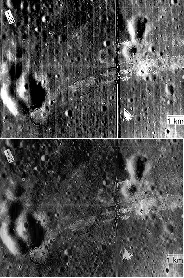
Figure 14.  Grayscale image of figure 11 (above), and the resulting image (below).

D.  Canvas Weave Modelling and Removal
     Next, the canvas pattern in this oil painting will be removed.  This canvas pattern is like superposition of sinusoids, so it is expected that the FT of this image will have dots.  Now,  the FT was taken, as shown in figure16.  There are dots as expected.  The mask is designed in such a way that the dots will be blocked out.  The mask and the FT was multiplied, and the absolute value of the inverse fft was obtained to get the modified image.  Figure 18 shows the comparison of the image before and after filtering, and it is clear that the weave pattern is removed.

Figure 15.  Detail of an oil painting from the UP Vargas 

Museum Collection.

Figure 16. FT of the oil painting image.

Figure 17.  Masking of the FT of the oil painting.

Figure 18.  Grayscale of the oil painting (above) and the resulting 

filtered image (below).

Figure 19.  Inverse color of the filter used for the filtering of the oil canvas.

Figure 20.  FT of figure 19.

Figure 21. Logarithm of the FT of the filter.

     Next, the question is: given the filter mask, how will you get the canvas weave pattern?  Answer: Get its FT!!  So, I edited the mask in Paint and reverted the colors.  Then, the FT was obtained.  Because the FT is small, I used the log value of the FT, as shown in figure 21.  The resulting FT is somewhat similar to the canvas pattern on the image.

     I would give myself a 10/10 for this activity.  I had given all required outputs and explained the results.  I would like to thank Joseph Raphael Bunao and Ma'am Jing for the helpful discussions.

Properties of the 2D Fourier Transform

     In this activity,  some properties of the 2D Fourier Transform (FT) will be demonstrated.  According to the Fourier theorem, any signal can be decomposed into superposition of sinusoids.   Fourier Transform is a linear transformation, that is, rotation of the sinusoids would also result into rotation in the frequency domain.

A.  Familiarization of FT of different 2D patterns
  

     Using Paint, images of a square, annulus (donut), square annulus, two slits along the x-axis that is symmetric about the center spanning the whole y-axis, and two dots symmetric about the center were created.  Then, these images were loaded into Scilab using the gray_imread() function.  The function fft2() was applied, then the absolute value was obtained using abs().  The function fftshift() was applied to the absolute value to center the FT.  Figure 1 shows the 2D images and their corresponding FT.

        

  

Figure 1.  Different 2D patterns (left) and their corresponding FT (right).

     Notice that if the 2D patterns are apertures, their corresponding FT is the interference pattern of the  monochromatic light that passes through it.  

B.  Anamorphic Property of the Fourier Transform

     In Scilab, a 2D sinusoid was created with varying frequencies.  From figures 2-4, the frequency is increased.  Notice that as the frequency is increased, the peaks in the Fourier domain goes farther from the center.  From this, we can say that lower  frequencies are near the center, and the higher frequencies are farther away.  This knowledge is helpful in noise filtering.  If one knows whether the needed data is in low frequency or high frequency, he/she could detect if the data is full of noise.

Figure 2.  A sinusoid with frequency equal to 4 (left) and its FT (right).

Figure 3.  A sinusoid with frequency equal to 8 (left) and its FT (right).

Figure 4. A sinusoid with frequency equal to 12 (left) and its FT (right).

     Next, a real image was simulated by adding a constant bias on the sinusoid.  Figure 5 shows the image of the FT.  Notice the addition of a peak at the center.  This peak corresponds to the added bias on the sinusoid.

Figure 5.  FT of a sinusoid with bias equal to 0.5 and frequency of 12.

     Next, the sinusoid patterns were rotated, and their corresponding FT were obtained.  Notice that the rotation of the sinusoids resulted also in the rotation in the Fourier domain.  

Figure 6. A sinusoid pattern rotated at 30 degrees (left) and its FT (right).

Figure 7.  A sinusoid pattern rotated at 60 degrees (left) and its FT (right).

Figure 8.  A sinusoid pattern rotated at 90 degrees (left) and its FT (right).

     What will happen to the FT if we created different patterns of sinusoids?  The prediction is that, since the FT is a linear transformation, the corresponding FT will the the superposition of the individual patterns.  It is seen from figures 2-4 that the FT of a corrugated roof running at the x-axis are two dots symmetric along the x-axis.  The pattern created is a product of two corrugated roofs, one running at the x-axis and the other at the y-axis.  As expected, the FT is the combination of the individual FTs.  A sinusoid rotated at 30 degrees was added to the pattern at figure 9.  Its FT is expected to be composed of four symmetric dots, and two tilted dots like in figure 6 (left).  As seen in figure 10, the FT is indeed what expected.

Figure 9.  A product of two corrugated roofs, one running on x-axis and the other

at the y-axis (right), and the corresponding FT (left).

Figure 10.   A product of two corrugated roofs, one running on x-axis and the other

at the y-axis (right), added with a sinusoid rotated at 30 degrees, and the corresponding FT (left).

     I would like to thank Ma'am Jing and Joseph Raphael Bunao for enlightening me on some points.  I would give myself a score of 9/10.  I produced all the required outputs, but I was not able to answer one question about finding the actual frequencies on an interferogram image.