SCILAB Basics 101

In this activity, I used Scilab 4.1.2 with Scilab Image Processing (SIP) toolbox. The advantage of using Scilab is that it is a free open source software that is comparable to Matlab. Like in Matlab, carrying out matrix operations in Scilab are simple.

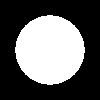
The goal of this activity is to create synthetic images that will be used later on for algorithm testing or simulating optical phenomena in imaging systems. The code for a circular aperture is given in the manual and shown below.

Fig. 1 Circular aperture of radius 0.7

code:

//circular apperture

nx = 100;

ny = 100; //defines the number of elements along x and y

x = linspace(-1,1,nx); //defines the range

y = linspace(-1,1,ny);

[X,Y] = ndgrid(x,y); //creates two 2-D arrays of x and y coordinates

r= sqrt(X.^2 + Y.^2); //note element-per-element squaring of X and Y

A = zeros (nx,ny);

A (find(r <0.7))> //radius of the aperture

imwrite(A, 'C:\Users\May Ann\Desktop\circularapp.jpg'); //saving of the image

imshow (A,[]);

We were asked to create synthetic images of a centered square aperture, sinusoid along the x-direction (corrugated roof), grating along the x-direction, annulus, and a circular aperture with graded transparency (gaussian transparency). Below are my outputs.

The framework of all succeeding codes is from the code given in the manual. I tried replacing some functions to achieve other required outputs.

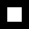
Figure 2. Centered square aperture with side of 0.5

code:

//square

nx = 100;

ny = 100; //defines the number of elements along x and y

x = linspace(-1,1,nx); //defines the range

y = linspace(-1,1,ny);

[X,Y] = ndgrid(x,y); //creates two 2-D arrays of x and y coordinates

A = zeros(nx, ny)

A(find((X>=-0.5 & X<=0.5) & (Y>=-0.5 & Y<=0.5))) = 1; // defines the square aperture

imwrite(A,'C:\Users\May Ann\Desktop\square.jpg');

imshow(A,[]);

Figure 3. Sinusoid along x-axis (Corrugated roof)

code:

//sinusoid

nx = 100;

ny = 100; //defines the number of elements along x and y

x = linspace(-1,1,nx); //defines the range

y = linspace(-1,1,ny);

[X,Y] = ndgrid(x,y); //creates two 2-D arrays of x and y coordinates

r = sin(5*%pi*X); //defines the sine function with frequency = 5/2

imwrite(r, 'C:\Users\May Ann\Desktop\sinusoid.jpg');

imshow(r, []);

Figure 4. Grating along x

code:

//grating

nx = 100;

ny = 100; //defines the number of elements along x and y

x = linspace(-1,1,nx); //defines the range

y = linspace(-1,1,ny);

[X,Y] = ndgrid(x,y); //creates two 2-D arrays of x and y coordinates

r = sin(2*%pi*10*X); //creates a sine function with f = 10

A = zeros(nx, ny);

A(find(r <0.3))= class="Apple-style-span" color="#009900">// defines the grating

imshow(A,[]);

imwrite(A,'C:\Users\May Ann\Desktop\grating.jpg');

Figure 5. Annulus

code:

//annulus

nx = 100;

ny = 100; //defines the number of elements along x and y

x = linspace(-1,1,nx); //defines the range

y = linspace(-1,1,ny);

[X,Y] = ndgrid(x,y); //creates two 2-D arrays of x and y coordinates

r = sqrt(X.^2 + Y.^2); //note element-per-element squaring of X and Y

A = zeros (nx,ny);

A (find(r <> // defines outer circle

A (find(r<0.4)> //defines inner circle

imwrite(A, 'C:\Users\May Ann\Desktop\annulus.jpg');

imshow (A, []);

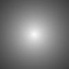
Figure 6. Circular aperture with

Gaussian transparency.

For a Gaussian, we expect that the center will have the maximum, as shown in figure 6.

code:

//graded circ aperture

nx = 100;

ny = 100; //defines the number of elements along x and y

x = linspace(-1,1,nx); //defines the range

y = linspace(-1,1,ny);

[X,Y] = ndgrid(x,y); //creates two 2-D arrays of x and y coordinates

r = sqrt(X.^2 + Y.^2);

s = exp(-r); // defines the Gaussian

imwrite(s, 'C:\Users\May Ann\Desktop\gradedcircapp.jpg');

imshow (s,[]);

I would like to thank Joseph Raphael Bunao for clarifying some syntax, and Celestino Andrew Borja for helping me out in saving the images. Also to Ma'am Jing for helping me in loading the SIP toolbox into Scilab.

I would give myself a score of 10 in this activity because I understood the lesson and produced all the required output. In addition, the images have good quality and are properly labeled.

Reference:

formula for Gaussian function: http://mathworld.wolfram.com/GaussianFunction.html