Wednesday, June 30, 2010

Area Estimation for Images with Defined Edges

This fourth activity is about area measurement.  Using Green's Theorem, the area of a defined contour can be obtained.  Green's Theorem says that the line integral of the boundary is equal to the area enclosed within that boundary. 


Using Paint, I created shapes of rectangle, square, and right triangle.  The background is color black, white for the shapes.  To know analytically the area of the shapes, I obtained the pixel coordinates of the edges. When counting for the pixel coordinates of the shape, consider only the white part of the image.  Using the formula for the area of these shapes, then we have the analytical area.  Below are the shapes I made, formulas for the area and the summary of the analytical area:


Figure 1 (a)

Figure 1 (b)

Figure 1 (c)

Figure 1.  Different shapes created using Paint.


Rectangle: A = Length*Width                    (1)
Square: A= Side*Side                               (2)
Right triangle = (1/2)(Base*Height)          (3)

            Table 1. Analytical areas of different shapes.
x1
y1
x2
y2
Length/Base
Height
Area
rectangle
104
103
299
198
195
95
18525
square
58
60
248
250
190
190
36100
triangle
72
39
272
262
200
223
22300


Note that the computed area are in terms of square pixels.

Now, let us compute for the area using Green's Theorem.  Using Scilab, load the image with the function 'imread'.  Then, get the contour of the shape using the function 'follow'.  This function obtains the coordinates of the border of the image.  It treats the '0' (black color) as background and the '1' (white) as the object.  This is the reason why when counting for the pixel coordinates of the object, one must consider only the white part.
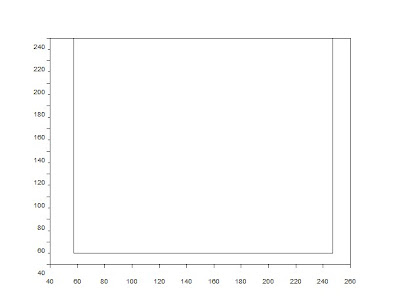
To check whether I got the correct set of coordinates, I plotted the values and are shown below:

Figure 2 (a)


Figure 2 (b)


Figure 2 (c)

Figure 2.  Contour plot for rectangle (a), square (b), and right triangle (c).

Then, I implemented the Green's Theorem in Scilab (see code below).  Here is the summary of the results:


Table 2.  Summary of the results.    
Analytical
Result
% difference
18525
18525
0
36100
36100
0
22300
22288
0.054


The % difference from the estimation of the area of the right triangle could be attributed to the slight deviation of its diagonal from being straight.


Figure 3.  Zoom in on the top part of the triangle.

Next, using Google Earth, I searched for the location of the Bahay ng Alumni.  Using the function printscreen, I pasted the image on Paint, as seen below:

Figure 4.  Aerial image of The Bahay ng Alumni (white part). 

I used the scale indicated on the map to convert the number of pixels in the image to its physical value.  The scale is:


145 ft = 259 pixels
1 square feet = 3.190535 square pixels
1square feet = 0.092903 square meter


Then, I edited the image in Paint.  I put a white layer on my object of interest, and then put a layer of black on the background that is close to the color white.  I do not have to color all of the background black. I could use the thresholding of the binary image conversion to rule out the background.  Below is the image of the edited version of the aerial view of the Bahay ng Alumni.

Figure 5. Edited image of the aerial view of the Bahay ng Alumni.

Then, on Scilab, I loaded the image and then converted it into grayscale.  Next, I converted it into a binary image with a threshold value of 1.  This would ensure that all of the background will be ruled out, as shown in Figure 5.


Figure 6.  Binary conversion of the edited image.
  
The area is obtained using the same method in computing for the area of different shapes.


 Table 3. Comparison of the area obtained to the area reported
Land Area (square meters)
Computed (square meters)
% error
Bahay ng Alumni
3000
2912.851
2.90%


The error could be from missing some pixels that are included in the object of interest.  The aerial image of The Bahay ng Alumni is not that sharp, so the edges are not well defined. I could only approximate as to where the edges are.

I would like to thank Joseph Raphael Bunao for listening to my rants as to why my code is not working.  :)  This kept me thinking on how to debug my code.

I would give myself a score of 10/10 because I got all the expected output and my results are quite good (error is less than 5%).  Also, I debugged my code without direct external help.  I independently found out the problems on my code and corrected them.

I enjoyed doing this activity because I understood the concepts and I got fairly good results. :)


Code:
//area estimation
stacksize(10000000);
img = imread('C:\Users\May Ann\Documents\May Ann\Acads\5th Year 1st Sem\Image Processing\A4 Area Estimation for Images with Defined Edges\bahay_alumni1.bmp');   //load image
gray_im = im2gray(img);        //convert image to grayscale
bw = im2bw(gray_im, 1);        //convert grayscale into binary
imshow(bw);
imwrite(bw, 'C:\Users\May Ann\Documents\May Ann\Acads\5th Year 1st Sem\Image Processing\A4 Area Estimation for Images with Defined Edges\bahay_alumni1bw.bmp');
[x,y] = follow(bw);                // makes a matrix of points that defines the object.
N = length(x)                      // number of points on the border of the contour
scf()
plot2d(x,y);
//imwrite([x,y],'C:\Users\May Ann\Documents\May Ann\Acads\5th Year 1st Sem\Image Processing\A4 Area Estimation for Images with Defined Edges\bahay_alumni_plot.bmp');

//implementation of Green's theorem
N = length(x);
n = N-1;
i = 1:n
p = sum(0.5*( x(i).*(y(i+1)) - x(i+1).*(y(i))));
q = 0.5*(x(N).*y(1) - x(1).*y(N));
Area = p + q


References:


Wednesday, June 23, 2010

Image Types and Fomats

An image, according to the dictionary, is a reproduction or imitation of a person or a thing. Other definition is that it is the optical counterpart of an object produced by an optical device. For our purposes, we will use the second definition.

There are four basic types of digitized images, binary, grayscale, indexed, and true color image.


Grayscale images. This image type has colors between 0 and 1 (black and white). Usually, this image type is stored as 8 bits, with 256 levels of gray from black to white. (See reference.)

Binary images. This image type has only two pixel values, 0 and 1. (Most binary representations has 0 as the black, and 1 as white, but some uses the reverse). Binary images are often used in many applications because it is simple to process. They are useful in analysis when only the silhouette of an object is needed to get all the information one wants about the object.
In conversion of images to binary, thresholding is typically done. For example, if the threshold value is set to 0.7, pixel values which are lower than that will have a value of 0, and higher pixel values will be set to 1. The choice of the threshold value can be based on the histogram of each pixel values of a grayscale image. (See reference.)

Indexed Images. In an indexed image, the actual image color for each pixel is the index into the palette or the color map. For example, a pixel's data corresponds to number 82, then the corresponding color is the 82nd in the color map. The color map comes in the file stored with the image. (See reference.)

True Color Images. A true color image has a very large number of colors, shades and hues. It has 256 shades of red, green, and blue for each pixel. Unlike in an indexed image, a true color image does not need a color map or palette. (See reference.)


Because of the emergence of advanced imaging techniques and devices, advanced image types emerged as well. Here are some examples:

Hyperspectral images. Hyperspectral imaging is a powerful and versatile means for sampling of broad intervals of the spectrum. Data acquisition are within the intervals of approximately 10nm, compared to 0.1 µm for broad bands. In this kind of imaging, each spatial element has a continuous spectrum that is used for analysis. Usually, hyperspectral imaging is used in satellite imaging.

High Dynamic Range Images. High dynamic range imaging is a linear kind of imaging. This means that each pixel value in the image is directly proportional to the amount of light intensity detected by the camera. This type of image stores pixel values that span the whole tonal range of real world scenes. As such, it is encoded in floating-point values that is stored with 32 bits per color channel. This encoding allows the largest range of values.

3D Images. The method of producing 3D images is similar to the way we see. Our left and right eye see slightly different images. Our brain fuses the two images, which allows us to see in three dimensions. In 3D imaging, two lenses placed that are placed side by side, are used to capture images. Then, filters or polarized light was used to ensure that only one image will be seen by each eye. Our brain fuses the two images together, creating an illusion of 3D.

Temporal Images or Videos. Videos are moving pictures. Typically, the number of still pictures per second ranges from 6 to 8. (See reference.)


I searched for images in the web and used imfinfo function in Scilab to display the image properties. Below are the examples of the different image types:


Figure 1. Example of a hyperspectral image.


Figure 2. Example of a high dynamic range image.


Figure 3. Example of a 3D image.


Figure 4. Example of an indexed image.


Figure 5. Example of a true color image.


Figure 6. Example of a binary image type.


Figure 7. Example of a gray scale image.


Image Formats

In image processing, the choice of image format to save your image is of vital importance.
Some image formats compresses the image and some valuable data were lost. This is called the
lossy image compression. In lossless image compression, no data were lost in compression and
each pixel information was conserved. Or, some recurring pixel pattern were replaced by a short
abbreviation.
There are several file types used today, namely the .tiff, .png, .jpeg/.jpg, .bmp, and . gif.

TIFF
Also known as Tagged Image File Format. This format is a type of lossless image compression.
Thus, a big file size is expected. Because of this, this file type is not used in web images, and
most web browsers do not display tiffs. However, tiff is useful in several editing and saving of
an image, because no data is lost in the process. (See reference.)

GIF
GIF stands for Graphics Interchange Format. It can display a maximum of 256 colors, which
makes it not good for photographic images. Its advantage is that it can be animated, and it is
often used in advertisements in the web. Another advantage is that it is a lossless format, similar
to tiff. It also requires a little amount of memory space. GIF can also be interlaced, meaning
different layers of an image can be loaded successively. In internet browsers, it gives an
impression of fast download.

PNG
Also known as Portable Network Graphics, this file type was invented in response to the payment
required to a software that supports a .gif file. This file type is also lossless, and it is superior to
.gif in using it in the web because it has 16 million colors, not just 256. (See reference.)
JPEG
Short for Joint Photographic Experts Group. It is designed specifically for photographs.
This format is capable of displaying millions of colors at once, which allows for the display
of complex hues that occurs in photographs. This file type could be lossy or lossless, depending on
the settings. An image can be saved to jpg without compression, which would mean a large file
size.For practicality, an image compression of 60% is used to optimize the size, without
compromising the quality of the image. (See reference.)

BMP
BMP, or the bitmap file type, is created by the Microsoft and IBM. Thus, it is bound to the
IBM compatible PC. All values stored in this format are in Intel format. This file type can be
lossy or lossless, depending on the settings. (See reference)
Now, we turn to the outputs of the procedures for Activity 3.
A true color image was converted into gray scale and binary image using gray_imread and im2bw functions in Scilab, respectively. The matrix size for both image conversion is 512x512.


Figure 8. Gray scale image conversion of a true color image.


Figure 9. Binary image conversion of a true color image.


Then, a grayscale image of the scanned old graph from Activity 1 was obtained. From this grayscale, a histogram of the pixel values was obtained using histplot function in Scilab.


Figure 10. Gray scale conversion of the scanned graph from
Activity 1.


Figure 11 (a)

Figure 11 (b)

Figure 11. Histogram plot of the pixel distribution of the scanned graph.
(a) histogram (b) zoom in


Here, we notice that there are small number of pixels up to 0.85. From this, the threshold value is set to 0.6. Notice that the image has good resolution for 0.5, 0.6, and 0.7 threshold value (right of 2nd column, and 3rd column). Lower threshold value shows blurring of the image, while higher threshold value shows artifacts in the graph. Dark areas caused by low quality scan of the image were highlighted.


Figure 12 (a) Threshold = 0.2


Figure 12 (b) Threshold = 0.3


Figure 12 (c) Threshold = 0.4


Figure 12 (d) Threshold = 0.5


Figure 12 (e) Threshold = 0.6


Figure 12 (f) Threshold = 0.7


Figure 12 (g) Threshold = 0.8


Figure 12 (h) Threshold = 0.9

Figure 12. Binary image conversion with increasing
threshold value.


Slow motion popping of a popcorn.
Video taken from here.


I would like to thank Cindyleen Kate Grieta, and Ma'am Jing for explaining
the meaning of the threshold value and histogram.

I would give myself a score of 8/10. All the outputs required for this activity were met,
except for the format of this blog report which is not in order.
(The images for advanced images were shown first, and the graphs with different
threshold values are not properly labeled)


References:
Merriam-Webster's 11th Collegiate Dictionary