Properties of the 2D Fourier Transform

     In this activity,  some properties of the 2D Fourier Transform (FT) will be demonstrated.  According to the Fourier theorem, any signal can be decomposed into superposition of sinusoids.   Fourier Transform is a linear transformation, that is, rotation of the sinusoids would also result into rotation in the frequency domain.

A.  Familiarization of FT of different 2D patterns
  

     Using Paint, images of a square, annulus (donut), square annulus, two slits along the x-axis that is symmetric about the center spanning the whole y-axis, and two dots symmetric about the center were created.  Then, these images were loaded into Scilab using the gray_imread() function.  The function fft2() was applied, then the absolute value was obtained using abs().  The function fftshift() was applied to the absolute value to center the FT.  Figure 1 shows the 2D images and their corresponding FT.

        

  

Figure 1.  Different 2D patterns (left) and their corresponding FT (right).

     Notice that if the 2D patterns are apertures, their corresponding FT is the interference pattern of the  monochromatic light that passes through it.  

B.  Anamorphic Property of the Fourier Transform

     In Scilab, a 2D sinusoid was created with varying frequencies.  From figures 2-4, the frequency is increased.  Notice that as the frequency is increased, the peaks in the Fourier domain goes farther from the center.  From this, we can say that lower  frequencies are near the center, and the higher frequencies are farther away.  This knowledge is helpful in noise filtering.  If one knows whether the needed data is in low frequency or high frequency, he/she could detect if the data is full of noise.

Figure 2.  A sinusoid with frequency equal to 4 (left) and its FT (right).

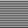
Figure 3.  A sinusoid with frequency equal to 8 (left) and its FT (right).

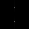
Figure 4. A sinusoid with frequency equal to 12 (left) and its FT (right).

     Next, a real image was simulated by adding a constant bias on the sinusoid.  Figure 5 shows the image of the FT.  Notice the addition of a peak at the center.  This peak corresponds to the added bias on the sinusoid.

Figure 5.  FT of a sinusoid with bias equal to 0.5 and frequency of 12.

     Next, the sinusoid patterns were rotated, and their corresponding FT were obtained.  Notice that the rotation of the sinusoids resulted also in the rotation in the Fourier domain.  

Figure 6. A sinusoid pattern rotated at 30 degrees (left) and its FT (right).

Figure 7.  A sinusoid pattern rotated at 60 degrees (left) and its FT (right).

Figure 8.  A sinusoid pattern rotated at 90 degrees (left) and its FT (right).

     What will happen to the FT if we created different patterns of sinusoids?  The prediction is that, since the FT is a linear transformation, the corresponding FT will the the superposition of the individual patterns.  It is seen from figures 2-4 that the FT of a corrugated roof running at the x-axis are two dots symmetric along the x-axis.  The pattern created is a product of two corrugated roofs, one running at the x-axis and the other at the y-axis.  As expected, the FT is the combination of the individual FTs.  A sinusoid rotated at 30 degrees was added to the pattern at figure 9.  Its FT is expected to be composed of four symmetric dots, and two tilted dots like in figure 6 (left).  As seen in figure 10, the FT is indeed what expected.

Figure 9.  A product of two corrugated roofs, one running on x-axis and the other

at the y-axis (right), and the corresponding FT (left).

Figure 10.   A product of two corrugated roofs, one running on x-axis and the other

at the y-axis (right), added with a sinusoid rotated at 30 degrees, and the corresponding FT (left).

     I would like to thank Ma'am Jing and Joseph Raphael Bunao for enlightening me on some points.  I would give myself a score of 9/10.  I produced all the required outputs, but I was not able to answer one question about finding the actual frequencies on an interferogram image. 

Fourier Transform Model of Image Formation

     Fourier Transform (FT) is a powerful tool in image processing.  It gives the spatial frequency, that is, for a signal of dimension X, the FT gives 1/X.  This activity is divided into four parts, so let us go through each part.

A.  Familiarization of the discrete FFT.

     Let us first familiarize ourselves with the discrete FT.  In Paint, create a 128x128 image of a white circle with a black background (shown in Figure 1.a).  Then, load this image in Scilab and convert it into grayscale.  fft2() was applied to the grayscale image.  Note that the result is a complex number array, and to see the intensity you need to take the absolute value by using the abs() function (shown in Figure 1.b). 

Figure 1.a Image of a 128x128 white circle with a black background.

     Notice that the result of the FFT looks like a black picture, but don't be fooled!! Look closely at the edges!  There is a very small white spot on the corners.  This represents the spatial frequency of the image.  Application of fftshift() centers the FFT, as seen in Figure 1.c.

Figure 2.b FFT of the image in Figure 1.a

Figure 1.c Shifted FFT of the image in Figure 1.a (circle)

Figure 1.d Application of the FFT to the

 image in Figure 1.a twice.

Figure 1. Output images for the familiarization of discrete FFT.

     Notice that the application of the FFT twice gives back the original image (see Figure 1.d). Now, let us apply the same procedure to a 128x128 image of a letter A (shown in Figure 2.a).

Figure 2. a) 128x128 image of a letter A.

Figure 2. b) Fourier Transform of the image in Figure 2.a

Figure 2.c) Shifted FFT of the image in Figure 2.a

Figure 2.d)   Application of the FFT to the

 image in Figure 2.a twice

Figure 2.  Output images for the familiarization of FFT using the image of letter a.

     The resulting image is inverted! What happened?? To understand this, let us look at the formula of the Fourier Transform:

 

     Equations 1 and 2 gives the formula for the FT and the inverse FT.  Based from these two equations, the application of the FT twice would introduce a negative sign on the output.  This explains the resulting inverted image.  To get the original image, use the inverse FT.  The inversion of the resulting image for the circle is not apparent because it is symmetric everywhere.

B.  Simulation of an imaging device.

     Now, let us go to the concept of convolution.  Given two functions f and g, their convolution gives out a function that is similar to both f and g.  In this part of the activity, we will simulate an imaging system.  For the object, a 128x128 image of the letters "VIP" was used.  For the imaging aperture, three centered circles of different radii were used. 

Figure 3.  A 128x128 image of letters VIP.

Figure 4.  Circles of different radii to act as an aperture

of the imaging system.

     

Figure 5.  Convolution of the object to circle of increasing radii (left to right).

     As can be observed, as the radius of the aperture is decreased, the image becomes blurry.  In an imaging system, the aperture acts as the limiter of the amount of light that will enter it.  As the radius of the aperture is decreased, the amount of information from the object also decreases.  This explains the image becoming blurry when the aperture is decreased.

C.   Template matching using correlation.

     The FT also has applications on template matching. Template matching is a pattern recognition technique that finds exact identical patterns in a scene [1]. Figure 6 shows the template used and the pattern to be detected.  Their FFT was obtained. Then, the complex conjugate of the resulting FFT of the template was obtained using the function conj().  Then, it was multiplied element per element to the FFT of the letter A.  Then, the FFT was obtained, as shown in Figure 7.

Figure 6.  Image used for pattern recognition (left) and the pattern to be 

recognized (right).

Figure 7.  Output of the template matching.  

     The bright spots on the resulting image represents the positions of the letter A.  So, the pattern to be detected is indeed detected.  :)

 D.  Edge detection using the convolution integral.

     This is like template matching in the previous activity, but this time, the ones to be detected are the edges.  Using Scilab, horizontal, vertical, and diagonal patterns were generated.  3x3 matrices whose total sum is zero were used to generate this patterns, as shown in Figure 8.

Figure 8.  3x3 matrix for horizontal (left), vertical (middle), and

diagonal (right) patterns.  

     Using the function imcorrcoef(), the patterns were convolved with the VIP image.  Figures 9-11 shows the output images of the convolution of the edges to the VIP image.  

Figure 9.  Horizontal edge detection. 

     Notice that horizontal lines are more pronounced than vertical and diagonal lines.  More so, the vertical lines are completely not seen.  This is because the horizontal and vertical lines are not related in any way.  There is a hint of diagonal lines because it has a horizontal component.

Figure 10.  Vertical edge detection.

     Notice that the vertical lines are more pronounced than the other lines.  This time, the horizontal lines are missing, and can be explained using the same argument in the horizontal edge detection.   Again, there is a hint of diagonal lines because it has a vertical component.    

Figure 11.  Diagonal edge detection.

     For the diagonal edge detection, diagonal, horizontal, and vertical lines are all apparent.  As been explained earlier, the diagonal has horizontal and vertical components. 

And that is the end of this activity. Hurray!!! :)

     Though I posted this blog late, I would still give my self a grade of 10/10.  I produced all the required outputs and I'm able to explain the results.  I would like to thank Ma'am Jing and Joseph Raphael Bunao for the useful conversations regarding the FFT. :D